Preface
This document compares the results for ten spectra across the
Spectral Analysis Shiny application, the online app luox by Manuel Spitschan, and
the free CIE S 026 alpha-opic Toolbox.
The main goal of this document is to validate the
Spectral Analysis application against the methods the CIE
has provided or already validated. We will look at results for
illuminance, α-opic irradiance, and
α-opic equivalent daylight (D65) illuminance. We will also
compare the irradiance (only with the toolbox) and
Correlated Color Temperature (CCT) and
Color-Rendering Index (CRI) (only with the luox app), which
are only available in one of the two validated sources. All three
sources offer more parameters, but those are either not part of both the
shiny application and a validated source or are derivatives of the
above-mentioned parameters. Some spectral data files had negative input
values (coming straight from the spectrometer export after measurement).
The Shiny app replaces these values with zero, whereas the
CIE toolbox gives an error for these values. Here, the
values were manually set to zero in the toolbox user input mask. The
luox app gives no error for negative values, but it is not
exactly known how the app deals with those values (see below under @sec-conclusion for more on that).
The results for the CIE Toolbox and luox
were taken on 21 October 2022 with their respective current
version at that date.
Table Preparation
The following code chunks prepare the tables shown below. The first chunk loads the necessary libraries:
Setup
#Setup code, data import, initial data selection to get to one comparison file
#read all libraries
library(dplyr)
#>
#> Attaching package: 'dplyr'
#> The following objects are masked from 'package:stats':
#>
#>     filter, lag
#> The following objects are masked from 'package:base':
#>
#>     intersect, setdiff, setequal, union
library(purrr)
library(ggplot2)
library(tibble)
library(readr)
library(stringr)
library(tidyr)
library(readxl)
library(magick)
#> Linking to ImageMagick 6.9.12.98
#> Enabled features: fontconfig, freetype, fftw, heic, lcms, pango, raw, webp, x11
#> Disabled features: cairo, ghostscript, rsvg
#> Using 4 threads
library(gt)
library(here)
#> here() starts at /home/runner/work/Spectran/Spectran
library(cowplot)
#>
#> Attaching package: 'cowplot'
#> The following object is masked from 'package:gt':
#>
#>     as_gtable

#Plottheme
theme_set(theme_cowplot(font_size = 10, font_family = "sans"))
The following chunk loads all data:
Data Import
#Data Import -------------------

##read all filenames and paths of spectra
spectra <-
  tibble(
    file_names = list.files("./Original_Spectra"),
    file_path = paste0("./Original_Spectra/", list.files("./Original_Spectra"))
    )

##read the csv-files to that spectra
spectra <-
  spectra %>%
  rowwise() %>%
  mutate(Spectrum = list(read_csv(file_path)))
#> Rows: 401 Columns: 2
#> ── Column specification ────────────────────────────────────────────────────────
#> Delimiter: ","
#> dbl (2): Wellenlaenge (nm), Bestrahlungsstaerke
#>
#> ℹ Use `spec()` to retrieve the full column specification for this data.
#> ℹ Specify the column types or set `show_col_types = FALSE` to quiet this message.
#> Rows: 401 Columns: 2
#> ── Column specification ────────────────────────────────────────────────────────
#> Delimiter: ","
#> dbl (2): Wellenlaenge (nm), Bestrahlungsstaerke (W/m^2)
#>
#> ℹ Use `spec()` to retrieve the full column specification for this data.
#> ℹ Specify the column types or set `show_col_types = FALSE` to quiet this message.

##create a name column
spectra <-
  spectra %>%
  mutate(spectrum_name = str_replace(file_names, ".csv", ""))

##read the results from the luox app
spectra <-
  spectra %>%
  rowwise() %>%
  mutate(
    luox = list(
      read_csv(
        paste0("./Results_Luox_2022-10-21/", spectrum_name,
               "/download-calc.csv")
        )
      )
    )
#> Rows: 35 Columns: 2
#> ── Column specification ────────────────────────────────────────────────────────
#> Delimiter: ","
#> chr (1): Condition
#> dbl (1): Bestrahlungsstaerke (W/m^2)
#>
#> ℹ Use `spec()` to retrieve the full column specification for this data.
#> ℹ Specify the column types or set `show_col_types = FALSE` to quiet this message.

##read the results from the shiny app
###filepath
excel_file_path <- function(spectrum_name) {
  paste0(
    "./Results_ShinyApp/",
    {{ spectrum_name }},
    "/",
    {{ spectrum_name }},
    "_9_2022-10-20.xlsx"
    )
}
###list for each worksheet in the excel-file
spectra <-
  spectra %>%
  rowwise() %>%
  mutate(
    shiny = list(
      list(
        Radiometrie = read_xlsx(
          excel_file_path(spectrum_name),
          sheet = "Radiometrie"
          ),
        Photometrie = read_xlsx(
          excel_file_path(spectrum_name),
          sheet = "Photometrie"
          ),
        Alpha = read_xlsx(
          excel_file_path(spectrum_name),
          sheet = "Alpha-opisch"
          )
        )
      )
    )

##read the results from the CIE toolbox
spectra <-
  spectra %>%
  rowwise() %>%
  mutate(
    toolbox = list(
      read_xlsx(
        paste0(
          "./Results_CIE_Toolbox/",
          spectrum_name,
          "/CIE S 026 alpha-opic Toolbox.xlsx"
          ),
        sheet = "Outputs"
        )
      )
    )
#> New names:
#> New names:
#> New names:
#> New names:
#> New names:
#> New names:
#> New names:
#> New names:
#> New names:
#> New names:
#> • `` -> `...2`
#> • `` -> `...3`
#> • `` -> `...4`
#> • `` -> `...5`
The following chunk takes the relevant data for comparison out from the sources and puts them into one table per comparison spectrum:
Initial Data wrangling
#Initial Data wrangling -------------------
##take the relevant datapoints from the luox results
### the relevant data in the luox results are in column 2, rows 1, 6 to 15, 22,
### and 24
locations_luox <- c(1, 6:15, 22, 24)
spectra <-
  spectra %>%
  rowwise() %>%
  mutate(
    excerpt = list(
      tibble(
        Name = luox %>% pull(1) %>% .[locations_luox],
        Results_luox = luox %>% pull(2) %>% .[locations_luox]
        )
      )
    )

###Add a row for irradiance, which is missing in the luox output
spectra <-
  spectra %>%
  mutate(
    excerpt = list(
      rbind(
        excerpt[1:11,],
        c("Irradiance (mW ⋅ m⁻²)", NA),
        excerpt[12:13,]
        )
      ),
    excerpt = list(
      excerpt %>% mutate(Results_luox = as.numeric(Results_luox))
    )
    )

##extract the relevant datapoints from the shiny app
### the relevant data in the shiny app results are in the list
### - "Photometrie", column 3, row 1,
### - "Alpha", column 3 to 7, row 1 to 2 (the order has to be adjusted in order
###to match the luox data frame)
### - "Radiometrie, column 3, row 1,
### - "Photometrie", column 3, row 4 to 5
shiny_extract <- function(data, sheet, column = Wert, rows) {
  data %>% .[[sheet]] %>% pull({{ column }}) %>% .[rows]
}
spectra <-
  spectra %>%
  rowwise() %>%
  mutate(
    excerpt = list(
      cbind(
        excerpt[1],
        tibble(
        Results_shiny = as.numeric(
          c(
            shiny_extract(
              data = shiny, sheet = "Photometrie", rows = 1),
            shiny_extract(
              data = shiny, sheet = "Alpha", column = "Cyanopsin", rows = 2),
            shiny_extract(
              data = shiny, sheet = "Alpha", column = "Chloropsin", rows = 2),
            shiny_extract(
              data = shiny, sheet = "Alpha", column = "Erythropsin", rows = 2),
            shiny_extract(
              data = shiny, sheet = "Alpha", column = "Rhodopsin", rows = 2),
            shiny_extract(
              data = shiny, sheet = "Alpha", column = "Melanopsin", rows = 2),
            shiny_extract(
              data = shiny, sheet = "Alpha", column = "Cyanopsin", rows = 1),
            shiny_extract(
              data = shiny, sheet = "Alpha", column = "Chloropsin", rows = 1),
            shiny_extract(
              data = shiny, sheet = "Alpha", column = "Erythropsin", rows = 1),
            shiny_extract(
              data = shiny, sheet = "Alpha", column = "Rhodopsin", rows = 1),
            shiny_extract(
              data = shiny, sheet = "Alpha", column = "Melanopsin", rows = 1),
            shiny_extract(
              data = shiny, sheet = "Radiometrie", rows = 1),
            shiny_extract(
              data = shiny, sheet = "Photometrie", rows = c(4, 5))
            )
          )
        ),
        excerpt[2]
        )
      )
  )

##extract the relevant datapoints from the CIE Toolbox
### the relevant data in the toolbox are in
### column 3, row 14
### column 1 to 5, row 20-> needs to be multiplied by a factor of 1000 to be in
### mW, to which the other sources are scaled.
### column 1 to 5, row 32
### column 1, row 14 -> needs to be multiplied by a factor of 1000 to be in mW,
### to which the other sources are scaled.
spectra <-
  spectra %>%
  mutate(
    excerpt = list(
      cbind(
        excerpt,
        tibble(
          Results_toolbox = as.numeric(
            c(
              toolbox %>% pull(3) %>% .[14],
              toolbox %>% {as.vector(.[20,])} %>% as.numeric %>%
                magrittr::multiply_by(1000),
              toolbox %>% {as.vector(.[32,])},
              toolbox %>% pull(1) %>% .[14] %>% as.numeric %>%
                magrittr::multiply_by(1000),
              NA, NA
              )
            )
          )
        )
      )
    )
The following chunk transforms the comparison tables for all spectra into one comprehensive table.
Putting the table together
#Putting the table together -------------------
##create a function that calculates the relative difference between the shiny
##app-results, and another source
Deviation <- function(Results, Results2){
  if(!is.na({{ Results }}) & !is.na({{ Results2 }})){
  res <- 1- {{ Results }} / {{ Results2 }}
  res2 <- vec_fmt_scientific(res)
  if(res < 0) {
    paste0('<div style="color:red">', res2, '</div>')
  }
  else if(res == 0 ) {
    paste0('<div style="color:green">', res2, '</div>')
  }
  else {
    paste0('<div style="color:blue">', res2, '</div>')
  }

  }
  else NA
}

##new dataframe, unnested data, columns for relative difference
Results <-
  spectra %>%
  select(spectrum_name, excerpt) %>%
  unnest(excerpt) %>%
  rowwise() %>%
  mutate(Dev_luox = Deviation(Results_luox, Results_shiny),
         Dev_toolbox = Deviation(Results_toolbox, Results_shiny)
         )

##pivoting the dataframe wider, so that each spectrum has only one row
Results <-
  Results %>%
  pivot_wider(
    id_cols = spectrum_name,
    names_from = Name,
    values_from = c(Results_shiny:Dev_toolbox),
    names_sep = "."
    )

##adding a placeholder for the spectrum picture, with the filepath
###filepath
pdf_file_path <- function(spectrum_name) {
  paste0("<img src='Results_ShinyApp/",
    {{ spectrum_name }},
    "/",
    {{ spectrum_name }},
    "_1_Radiometrie_2022-10-20.png' style=\'height:80px;\'>"
    )
}
###splicing the dataframes together
Results <- cbind(Results[,1], as_tibble_col(
  pdf_file_path(spectra$spectrum_name), column_name = "Picture"), Results[,-1])
The next chunk prepares the table output in a flexible way:
Setting the Table up
#setting the table up -------------------

##names for the merging
merging_names <- spectra$excerpt[[1]]$Name
merging_names2 <- spectra$excerpt[[1]]$Name %>% str_replace("\\(", "<br>\\(")

##column names for renaming
col_names <- paste0("Results_shiny.", merging_names)
##creating a list with one entry per variable, named after the column name (to
##be renamed later)
renaming <- rbind(merging_names2)
names(renaming) <- col_names
renaming <- renaming %>% as.list()
renaming <- map(renaming, md)

#creating a list with cells not to format by decimals
number_fmt_col <-
  Results %>% select(!starts_with("Dev") & !Picture & !spectrum_name) %>%
  names()

##function that does the merging
merging <- function(data, Name, condition = "difference") {
  if(condition == "difference"){
  data %>% cols_merge(columns = ends_with(Name, ignore.case = FALSE),
             pattern = "<div style='color:lightgrey'>shiny:</div>{1}<div
             style='color:lightgrey'>luox:</div>{4}<div style='color:lightgrey'>
             toolbox:</div>{5}")
  }
  else {
      data %>% cols_merge(columns = ends_with(Name, ignore.case = FALSE),
             pattern = "<div style='color:lightgrey'>shiny:</div>{1}<div
             style='color:lightgrey'>luox:</div>{2}<div style='color:lightgrey'>
             toolbox:</div>{3}")
  }
}

#creating a function for the gt table
comparison_table <- function(tt_text, fn_text, condition) {
gtobj <- Results %>%
  gt(rowname_col = c("spectrum_name")) %>%
  tab_header(title = md(paste0("**Validation Results: ",tt_text , "**"))) %>%
  tab_footnote(footnote = fn_text)

for(i in seq_along(merging_names)) {
  gtobj <- gtobj %>% merging(merging_names[i], condition = condition)
}

gtobj <- gtobj %>%
  fmt_markdown(columns = everything()) %>%
  fmt_number(
    columns = all_of(number_fmt_col),
    decimals = 3,
    sep_mark = "",
    pattern = "{x}<br>"
    ) %>%
  cols_align(align = "center") %>%
  cols_label(.list = renaming) %>%
  sub_missing(missing_text = md("---<br>")) %>%
  cols_width(
    Picture ~px(150),
    everything() ~ px(80)
  ) %>%
  opt_align_table_header(align = "left") %>%
  tab_options(table.font.size = "9px")

gtobj

}
Results
This section shows the validation results in two tables. The first
table shows the results for the Shiny App per spectrum and
parameter alongside the relative difference of the respective results
from the luox app and the CIE Toolbox. The
second table shows all results per spectrum and parameter. Note that the
Shiny App does not provide a CRI [Ra] for the
artificial EE_Spektrum and the LED_4000K_2,
because they exceed the CIE limits for calculation.
Creating the gt Table
#creating the gtable -------------------

#text for the subtitle
fn_text <-
  md(paste0(
    "The first number in every cell shows the Result from the *Shiny* app, ",
    "<br>the second number the **relative** difference of the respective ",
    "result from the *luox* app, <br>whereas the third number shows the same ",
    "for the result from the *CIE S026 Toolbox*. <br><a style='color:green'>",
    "green</a> values indicate a zero difference, <a style='color:red'>red</a>",
    " a negative difference, and <a style='color:blue'>blue</a> a positive ",
    "difference. <br>All *Shiny* values are rounded to three decimals. <br>",
    "Missing values or pairwise comparisons are indicated by a ---."))

tt_text <- "Relative Differences"
comparison_table(tt_text, fn_text, condition = "difference")| Validation Results: Relative Differences | |||||||||||||||
| Picture | Illuminance (lx) |
S-cone-opic irradiance (mW ⋅ m⁻²) |
M-cone-opic irradiance (mW ⋅ m⁻²) |
L-cone-opic irradiance (mW ⋅ m⁻²) |
Rhodopic irradiance (mW ⋅ m⁻²) |
Melanopic irradiance (mW ⋅ m⁻²) |
S-cone-opic EDI (lx) |
M-cone-opic EDI (lx) |
L-cone-opic EDI (lx) |
Rhodopic EDI (lx) |
Melanopic EDI (lx) |
Irradiance (mW ⋅ m⁻²) |
CCT (K) - Robertson, 1968 |
Colour Rendering Index [Ra] | |
|---|---|---|---|---|---|---|---|---|---|---|---|---|---|---|---|
| EE_Spektrum | 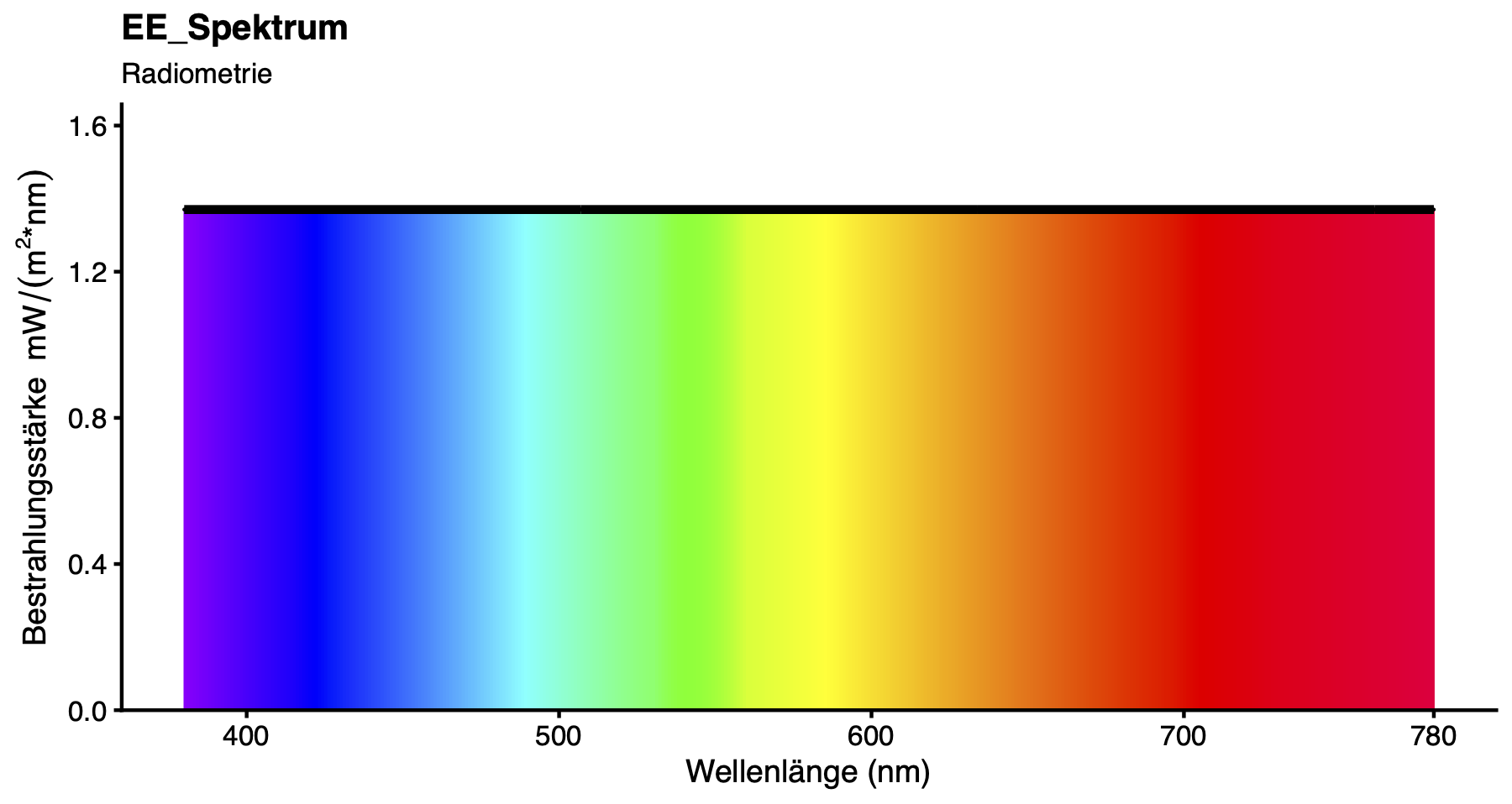 |
shiny: 100.000luox:
−2.93 × 10⁻⁶
toolbox:
−2.27 × 10⁻⁶
|
shiny: 75.641luox:
0.00
toolbox:
4.88 × 10⁻¹⁵
|
shiny: 139.676luox:
0.00
toolbox:
7.33 × 10⁻¹⁵
|
shiny: 163.891luox:
2.51 × 10⁻⁹
toolbox:
3.77 × 10⁻¹⁵
|
shiny: 133.005luox:
0.00
toolbox:
3.00 × 10⁻¹⁵
|
shiny: 120.131luox:
0.00
toolbox:
4.66 × 10⁻¹⁵
|
shiny: 92.550luox:
−1.27 × 10⁻⁵
toolbox:
−1.27 × 10⁻⁵
|
shiny: 95.945luox:
1.81 × 10⁻⁵
toolbox:
1.81 × 10⁻⁵
|
shiny: 100.614luox:
4.77 × 10⁻⁶
toolbox:
4.77 × 10⁻⁶
|
shiny: 91.747luox:
2.47 × 10⁻⁶
toolbox:
2.47 × 10⁻⁶
|
shiny: 90.583luox:
9.94 × 10⁻⁶
toolbox:
9.94 × 10⁻⁶
|
shiny: 549.443luox:
—
toolbox:
7.44 × 10⁻¹⁵
|
shiny: 5453.666luox:
−1.78 × 10⁻¹⁵
toolbox:
— |
shiny:
—luox:
—
toolbox:
— |
| Fluoreszenz_NW | 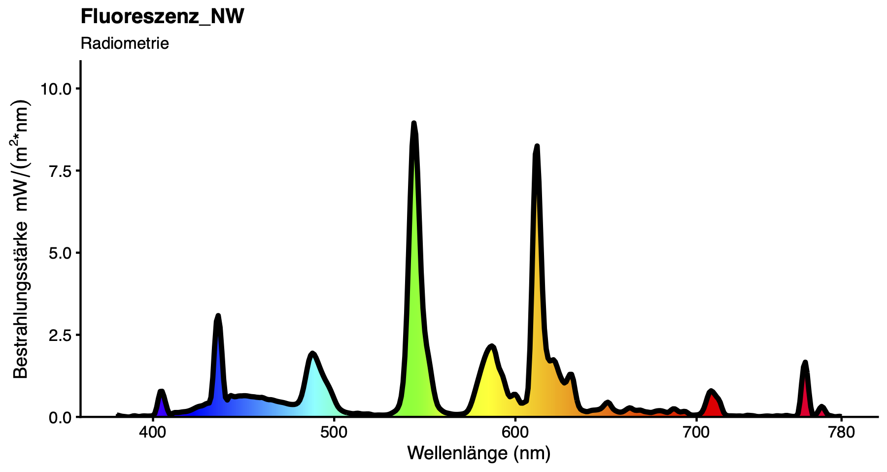 |
shiny: 100.000luox:
−2.93 × 10⁻⁶
toolbox:
−2.27 × 10⁻⁶
|
shiny: 40.235luox:
0.00
toolbox:
5.55 × 10⁻¹⁶
|
shiny: 125.328luox:
0.00
toolbox:
3.33 × 10⁻¹⁶
|
shiny: 161.847luox:
4.62 × 10⁻¹⁰
toolbox:
3.89 × 10⁻¹⁵
|
shiny: 90.644luox:
4.46 × 10⁻⁸
toolbox:
1.55 × 10⁻¹⁵
|
shiny: 71.312luox:
8.36 × 10⁻⁸
toolbox:
1.44 × 10⁻¹⁵
|
shiny: 49.229luox:
−1.27 × 10⁻⁵
toolbox:
−1.27 × 10⁻⁵
|
shiny: 86.089luox:
1.81 × 10⁻⁵
toolbox:
1.81 × 10⁻⁵
|
shiny: 99.360luox:
4.77 × 10⁻⁶
toolbox:
4.77 × 10⁻⁶
|
shiny: 62.526luox:
2.51 × 10⁻⁶
toolbox:
2.47 × 10⁻⁶
|
shiny: 53.772luox:
1.00 × 10⁻⁵
toolbox:
9.94 × 10⁻⁶
|
shiny: 293.442luox:
—
toolbox:
1.89 × 10⁻¹⁵
|
shiny: 3759.099luox:
7.57 × 10⁻⁸
toolbox:
— |
shiny: 83.077luox:
9.21 × 10⁻⁴
toolbox:
— |
| Fluoreszenz_WW |  |
shiny: 100.000luox:
−2.90 × 10⁻⁶
toolbox:
−2.27 × 10⁻⁶
|
shiny: 23.471luox:
0.00
toolbox:
2.78 × 10⁻¹⁵
|
shiny: 111.528luox:
1.84 × 10⁻⁹
toolbox:
5.11 × 10⁻¹⁵
|
shiny: 164.806luox:
1.78 × 10⁻⁸
toolbox:
3.33 × 10⁻¹⁵
|
shiny: 65.329luox:
4.15 × 10⁻⁷
toolbox:
8.88 × 10⁻¹⁶
|
shiny: 44.754luox:
9.02 × 10⁻⁷
toolbox:
1.11 × 10⁻¹⁵
|
shiny: 28.718luox:
−1.27 × 10⁻⁵
toolbox:
−1.27 × 10⁻⁵
|
shiny: 76.610luox:
1.81 × 10⁻⁵
toolbox:
1.81 × 10⁻⁵
|
shiny: 101.176luox:
4.79 × 10⁻⁶
toolbox:
4.77 × 10⁻⁶
|
shiny: 45.064luox:
2.88 × 10⁻⁶
toolbox:
2.47 × 10⁻⁶
|
shiny: 33.746luox:
1.08 × 10⁻⁵
toolbox:
9.94 × 10⁻⁶
|
shiny: 284.770luox:
—
toolbox:
2.22 × 10⁻¹⁵
|
shiny: 2676.108luox:
2.20 × 10⁻⁷
toolbox:
— |
shiny: 82.394luox:
2.29 × 10⁻⁴
toolbox:
— |
| Halogen | 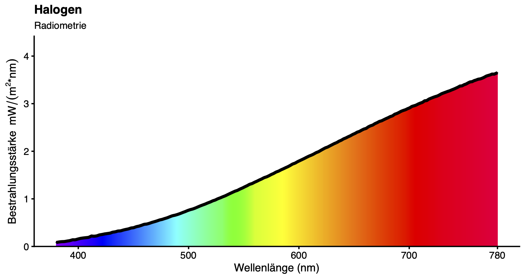 |
shiny: 100.000luox:
−2.93 × 10⁻⁶
toolbox:
−2.27 × 10⁻⁶
|
shiny: 22.648luox:
0.00
toolbox:
−2.22 × 10⁻¹⁶
|
shiny: 115.192luox:
0.00
toolbox:
3.33 × 10⁻¹⁶
|
shiny: 166.103luox:
4.51 × 10⁻⁹
toolbox:
3.11 × 10⁻¹⁵
|
shiny: 78.883luox:
0.00
toolbox:
2.33 × 10⁻¹⁵
|
shiny: 61.492luox:
0.00
toolbox:
2.00 × 10⁻¹⁵
|
shiny: 27.711luox:
−1.27 × 10⁻⁵
toolbox:
−1.27 × 10⁻⁵
|
shiny: 79.126luox:
1.81 × 10⁻⁵
toolbox:
1.81 × 10⁻⁵
|
shiny: 101.973luox:
4.77 × 10⁻⁶
toolbox:
4.77 × 10⁻⁶
|
shiny: 54.413luox:
2.47 × 10⁻⁶
toolbox:
2.47 × 10⁻⁶
|
shiny: 46.367luox:
9.94 × 10⁻⁶
toolbox:
9.94 × 10⁻⁶
|
shiny: 671.237luox:
—
toolbox:
1.33 × 10⁻¹⁵
|
shiny: 2714.135luox:
0.00
toolbox:
— |
shiny: 99.784luox:
−2.16 × 10⁻³
toolbox:
— |
| LED_2200K | 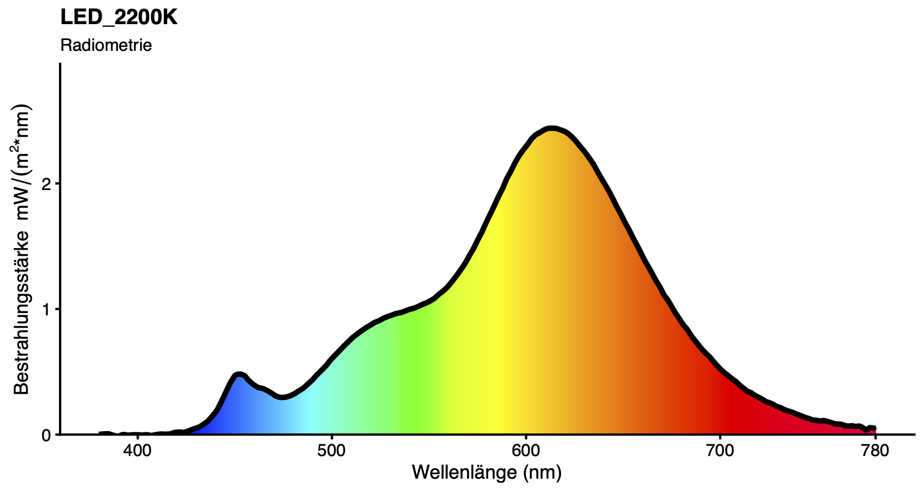 |
shiny: 100.000luox:
−2.71 × 10⁻⁶
toolbox:
−2.27 × 10⁻⁶
|
shiny: 15.044luox:
2.38 × 10⁻⁴
toolbox:
7.77 × 10⁻¹⁶
|
shiny: 109.249luox:
1.88 × 10⁻⁶
toolbox:
−1.78 × 10⁻¹⁵
|
shiny: 167.526luox:
1.28 × 10⁻⁶
toolbox:
2.00 × 10⁻¹⁵
|
shiny: 66.304luox:
1.23 × 10⁻⁵
toolbox:
4.44 × 10⁻¹⁶
|
shiny: 48.778luox:
2.14 × 10⁻⁵
toolbox:
2.00 × 10⁻¹⁵
|
shiny: 18.407luox:
2.26 × 10⁻⁴
toolbox:
−1.27 × 10⁻⁵
|
shiny: 75.044luox:
2.00 × 10⁻⁵
toolbox:
1.81 × 10⁻⁵
|
shiny: 102.846luox:
6.05 × 10⁻⁶
toolbox:
4.77 × 10⁻⁶
|
shiny: 45.736luox:
1.48 × 10⁻⁵
toolbox:
2.47 × 10⁻⁶
|
shiny: 36.780luox:
3.13 × 10⁻⁵
toolbox:
9.94 × 10⁻⁶
|
shiny: 329.187luox:
—
toolbox:
1.55 × 10⁻¹⁵
|
shiny: 2410.988luox:
4.61 × 10⁻⁶
toolbox:
— |
shiny: 87.665luox:
4.62 × 10⁻⁴
toolbox:
— |
| LED_4000K_1 | 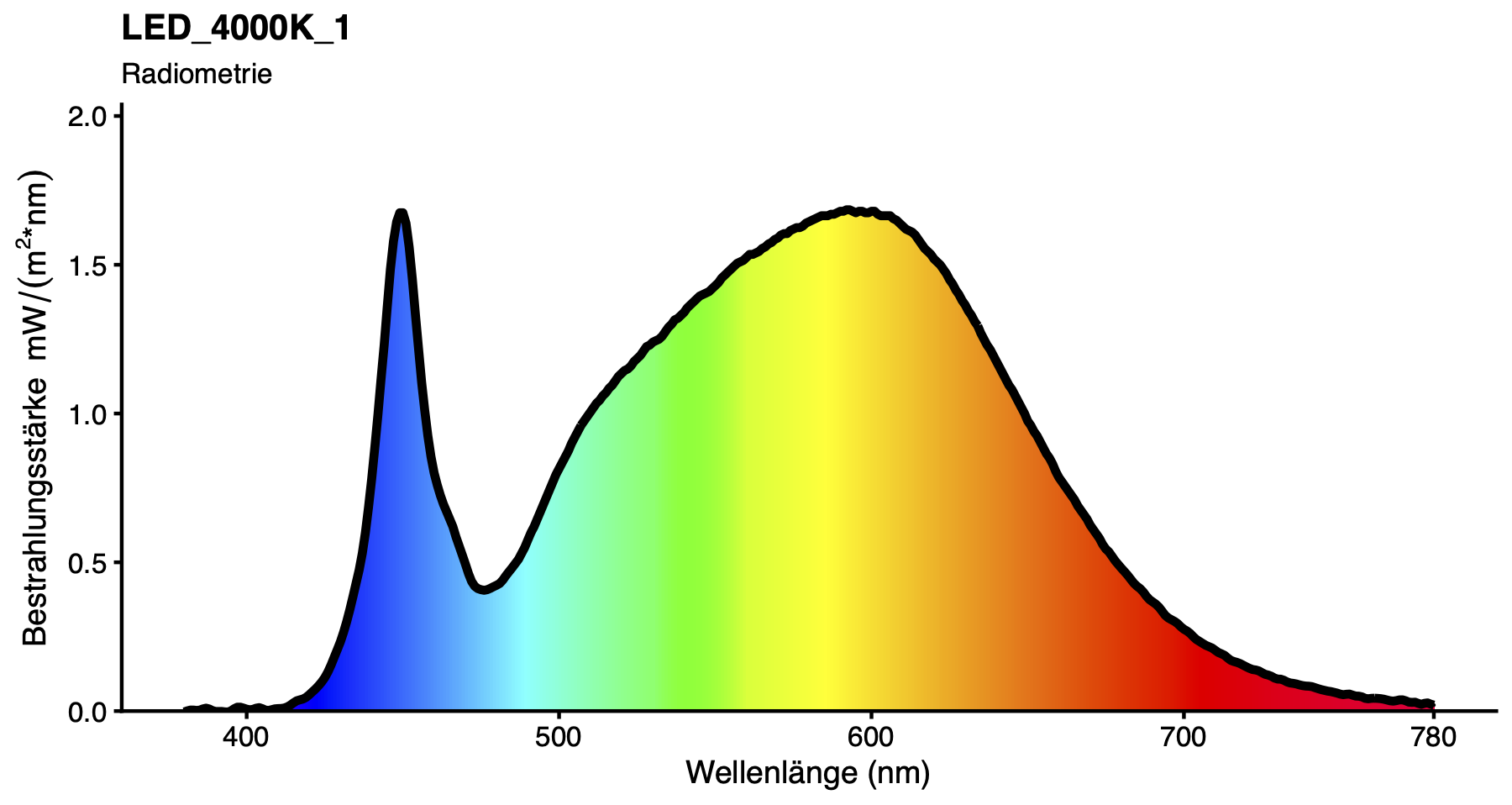 |
shiny: 100.000luox:
−2.92 × 10⁻⁶
toolbox:
−2.27 × 10⁻⁶
|
shiny: 39.460luox:
2.61 × 10⁻⁶
toolbox:
2.66 × 10⁻¹⁵
|
shiny: 126.303luox:
4.87 × 10⁻⁸
toolbox:
3.44 × 10⁻¹⁵
|
shiny: 162.057luox:
4.40 × 10⁻⁸
toolbox:
6.66 × 10⁻¹⁵
|
shiny: 93.656luox:
3.64 × 10⁻⁷
toolbox:
2.89 × 10⁻¹⁵
|
shiny: 74.836luox:
6.17 × 10⁻⁷
toolbox:
3.00 × 10⁻¹⁵
|
shiny: 48.281luox:
−1.01 × 10⁻⁵
toolbox:
−1.27 × 10⁻⁵
|
shiny: 86.759luox:
1.81 × 10⁻⁵
toolbox:
1.81 × 10⁻⁵
|
shiny: 99.489luox:
4.81 × 10⁻⁶
toolbox:
4.77 × 10⁻⁶
|
shiny: 64.603luox:
2.83 × 10⁻⁶
toolbox:
2.47 × 10⁻⁶
|
shiny: 56.429luox:
1.06 × 10⁻⁵
toolbox:
9.94 × 10⁻⁶
|
shiny: 300.094luox:
—
toolbox:
5.44 × 10⁻¹⁵
|
shiny: 3811.887luox:
5.90 × 10⁻⁷
toolbox:
— |
shiny: 82.085luox:
−4.92 × 10⁻⁴
toolbox:
— |
| LED_4000K_2 | 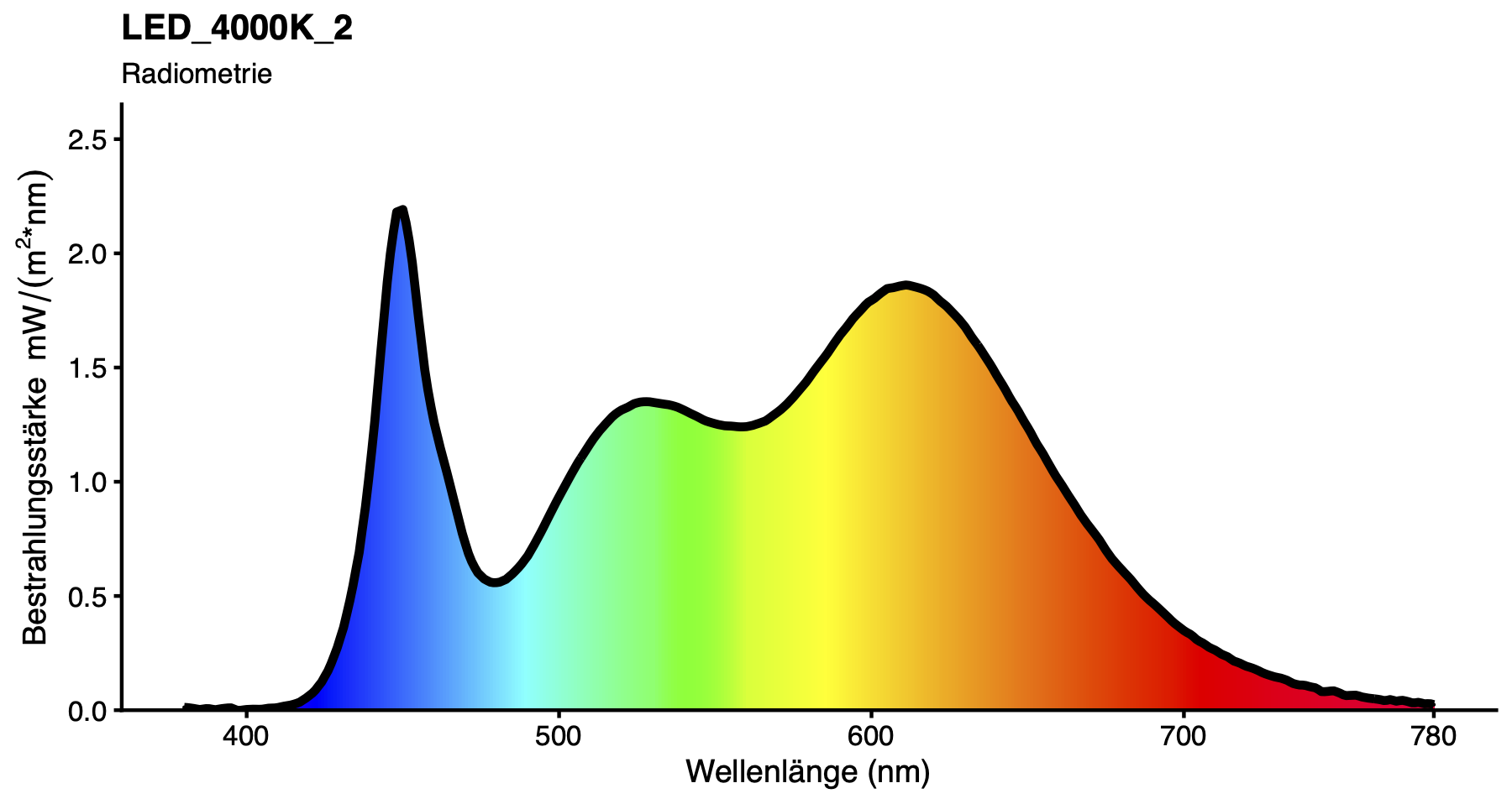 |
shiny: 100.000luox:
−2.93 × 10⁻⁶
toolbox:
−2.27 × 10⁻⁶
|
shiny: 54.816luox:
6.77 × 10⁻⁷
toolbox:
2.44 × 10⁻¹⁵
|
shiny: 127.856luox:
1.76 × 10⁻⁸
toolbox:
4.77 × 10⁻¹⁵
|
shiny: 164.399luox:
1.66 × 10⁻⁸
toolbox:
4.11 × 10⁻¹⁵
|
shiny: 106.315luox:
8.93 × 10⁻⁸
toolbox:
4.66 × 10⁻¹⁵
|
shiny: 90.404luox:
1.32 × 10⁻⁷
toolbox:
2.33 × 10⁻¹⁵
|
shiny: 67.069luox:
−1.20 × 10⁻⁵
toolbox:
−1.27 × 10⁻⁵
|
shiny: 87.825luox:
1.81 × 10⁻⁵
toolbox:
1.81 × 10⁻⁵
|
shiny: 100.926luox:
4.78 × 10⁻⁶
toolbox:
4.77 × 10⁻⁶
|
shiny: 73.336luox:
2.56 × 10⁻⁶
toolbox:
2.47 × 10⁻⁶
|
shiny: 68.168luox:
1.01 × 10⁻⁵
toolbox:
9.94 × 10⁻⁶
|
shiny: 338.823luox:
—
toolbox:
2.33 × 10⁻¹⁵
|
shiny: 3899.370luox:
1.72 × 10⁻⁷
toolbox:
— |
shiny:
—luox:
—
toolbox:
— |
| LED_6900K |  |
shiny: 100.000luox:
−2.92 × 10⁻⁶
toolbox:
−2.27 × 10⁻⁶
|
shiny: 93.998luox:
2.39 × 10⁻⁷
toolbox:
1.67 × 10⁻¹⁵
|
shiny: 145.326luox:
9.31 × 10⁻⁹
toolbox:
3.66 × 10⁻¹⁵
|
shiny: 161.924luox:
1.03 × 10⁻⁸
toolbox:
4.55 × 10⁻¹⁵
|
shiny: 144.972luox:
2.07 × 10⁻⁷
toolbox:
3.11 × 10⁻¹⁵
|
shiny: 131.440luox:
3.24 × 10⁻⁷
toolbox:
6.66 × 10⁻¹⁶
|
shiny: 115.010luox:
−1.24 × 10⁻⁵
toolbox:
−1.27 × 10⁻⁵
|
shiny: 99.826luox:
1.81 × 10⁻⁵
toolbox:
1.81 × 10⁻⁵
|
shiny: 99.407luox:
4.78 × 10⁻⁶
toolbox:
4.77 × 10⁻⁶
|
shiny: 100.001luox:
2.67 × 10⁻⁶
toolbox:
2.47 × 10⁻⁶
|
shiny: 99.110luox:
1.03 × 10⁻⁵
toolbox:
9.94 × 10⁻⁶
|
shiny: 351.290luox:
—
toolbox:
2.11 × 10⁻¹⁵
|
shiny: 7418.690luox:
1.36 × 10⁻⁶
toolbox:
— |
shiny: 93.878luox:
3.68 × 10⁻⁵
toolbox:
— |
| Nordhimmel |  |
shiny: 100.000luox:
−2.93 × 10⁻⁶
toolbox:
−2.27 × 10⁻⁶
|
shiny: 108.054luox:
−9.33 × 10⁻¹⁵
toolbox:
−2.00 × 10⁻¹⁵
|
shiny: 153.329luox:
0.00
toolbox:
4.44 × 10⁻¹⁵
|
shiny: 163.589luox:
1.91 × 10⁻⁹
toolbox:
2.11 × 10⁻¹⁵
|
shiny: 166.521luox:
0.00
toolbox:
5.44 × 10⁻¹⁵
|
shiny: 157.556luox:
0.00
toolbox:
6.66 × 10⁻¹⁶
|
shiny: 132.209luox:
−1.27 × 10⁻⁵
toolbox:
−1.27 × 10⁻⁵
|
shiny: 105.323luox:
1.81 × 10⁻⁵
toolbox:
1.81 × 10⁻⁵
|
shiny: 100.429luox:
4.77 × 10⁻⁶
toolbox:
4.77 × 10⁻⁶
|
shiny: 114.866luox:
2.47 × 10⁻⁶
toolbox:
2.47 × 10⁻⁶
|
shiny: 118.802luox:
9.94 × 10⁻⁶
toolbox:
9.94 × 10⁻⁶
|
shiny: 528.454luox:
—
toolbox:
3.44 × 10⁻¹⁵
|
shiny: 9317.532luox:
9.99 × 10⁻¹⁶
toolbox:
— |
shiny: 97.943luox:
−5.81 × 10⁻⁴
toolbox:
— |
| Norm_TL_6500K |  |
shiny: 100.000luox:
−2.93 × 10⁻⁶
toolbox:
−2.27 × 10⁻⁶
|
shiny: 81.711luox:
0.00
toolbox:
−4.44 × 10⁻¹⁶
|
shiny: 145.575luox:
0.00
toolbox:
7.77 × 10⁻¹⁶
|
shiny: 162.890luox:
2.06 × 10⁻⁹
toolbox:
2.11 × 10⁻¹⁵
|
shiny: 144.953luox:
0.00
toolbox:
9.99 × 10⁻¹⁶
|
shiny: 132.602luox:
0.00
toolbox:
3.44 × 10⁻¹⁵
|
shiny: 99.976luox:
−1.27 × 10⁻⁵
toolbox:
−1.27 × 10⁻⁵
|
shiny: 99.996luox:
1.81 × 10⁻⁵
toolbox:
1.81 × 10⁻⁵
|
shiny: 100.000luox:
4.77 × 10⁻⁶
toolbox:
4.77 × 10⁻⁶
|
shiny: 99.988luox:
2.47 × 10⁻⁶
toolbox:
2.47 × 10⁻⁶
|
shiny: 99.986luox:
9.94 × 10⁻⁶
toolbox:
9.94 × 10⁻⁶
|
shiny: 488.200luox:
—
toolbox:
−4.44 × 10⁻¹⁶
|
shiny: 6499.265luox:
0.00
toolbox:
— |
shiny: 99.991luox:
−8.92 × 10⁻⁵
toolbox:
— |
| The first number in every cell shows the Result from the Shiny app, the second number the relative difference of the respective result from the luox app, whereas the third number shows the same for the result from the CIE S026 Toolbox. green values indicate a zero difference, red a negative difference, and blue a positive difference. All Shiny values are rounded to three decimals. Missing values or pairwise comparisons are indicated by a —. |
|||||||||||||||
Creating the gt Table
#creating the gtable -------------------

#text for the subtitle
fn_text <- md("The first number in every cell shows the Result from the *Shiny*
              app, <br>the second number the result from the *luox* app, <br>
              whereas the third number shows the result from the *CIE S026
              Toolbox*. <br>All values are rounded to three decimals. <br>
              Missing values are indicated by a ---.")

tt_text <- "All Results"
comparison_table(tt_text, fn_text, condition = "")| Validation Results: All Results | |||||||||||||||
| Picture | Illuminance (lx) |
S-cone-opic irradiance (mW ⋅ m⁻²) |
M-cone-opic irradiance (mW ⋅ m⁻²) |
L-cone-opic irradiance (mW ⋅ m⁻²) |
Rhodopic irradiance (mW ⋅ m⁻²) |
Melanopic irradiance (mW ⋅ m⁻²) |
S-cone-opic EDI (lx) |
M-cone-opic EDI (lx) |
L-cone-opic EDI (lx) |
Rhodopic EDI (lx) |
Melanopic EDI (lx) |
Irradiance (mW ⋅ m⁻²) |
CCT (K) - Robertson, 1968 |
Colour Rendering Index [Ra] | |
|---|---|---|---|---|---|---|---|---|---|---|---|---|---|---|---|
| EE_Spektrum | |
shiny: 100.000luox: 100.000
toolbox: 100.000 |
shiny: 75.641luox: 75.641
toolbox: 75.641 |
shiny: 139.676luox: 139.676
toolbox: 139.676 |
shiny: 163.891luox: 163.891
toolbox: 163.891 |
shiny: 133.005luox: 133.005
toolbox: 133.005 |
shiny: 120.131luox: 120.131
toolbox: 120.131 |
shiny: 92.550luox: 92.551
toolbox: 92.551 |
shiny: 95.945luox: 95.943
toolbox: 95.943 |
shiny: 100.614luox: 100.614
toolbox: 100.614 |
shiny: 91.747luox: 91.747
toolbox: 91.747 |
shiny: 90.583luox: 90.582
toolbox: 90.582 |
shiny: 549.443luox:
—
toolbox: 549.443 |
shiny: 5453.666luox: 5453.666
toolbox:
— |
shiny:
—luox: 95.250
toolbox:
— |
| Fluoreszenz_NW | |
shiny: 100.000luox: 100.000
toolbox: 100.000 |
shiny: 40.235luox: 40.235
toolbox: 40.235 |
shiny: 125.328luox: 125.328
toolbox: 125.328 |
shiny: 161.847luox: 161.847
toolbox: 161.847 |
shiny: 90.644luox: 90.644
toolbox: 90.644 |
shiny: 71.312luox: 71.312
toolbox: 71.312 |
shiny: 49.229luox: 49.230
toolbox: 49.230 |
shiny: 86.089luox: 86.087
toolbox: 86.087 |
shiny: 99.360luox: 99.359
toolbox: 99.359 |
shiny: 62.526luox: 62.526
toolbox: 62.526 |
shiny: 53.772luox: 53.771
toolbox: 53.771 |
shiny: 293.442luox:
—
toolbox: 293.442 |
shiny: 3759.099luox: 3759.099
toolbox:
— |
shiny: 83.077luox: 83.000
toolbox:
— |
| Fluoreszenz_WW | |
shiny: 100.000luox: 100.000
toolbox: 100.000 |
shiny: 23.471luox: 23.471
toolbox: 23.471 |
shiny: 111.528luox: 111.528
toolbox: 111.528 |
shiny: 164.806luox: 164.806
toolbox: 164.806 |
shiny: 65.329luox: 65.329
toolbox: 65.329 |
shiny: 44.754luox: 44.754
toolbox: 44.754 |
shiny: 28.718luox: 28.718
toolbox: 28.718 |
shiny: 76.610luox: 76.608
toolbox: 76.608 |
shiny: 101.176luox: 101.176
toolbox: 101.176 |
shiny: 45.064luox: 45.064
toolbox: 45.064 |
shiny: 33.746luox: 33.746
toolbox: 33.746 |
shiny: 284.770luox:
—
toolbox: 284.770 |
shiny: 2676.108luox: 2676.108
toolbox:
— |
shiny: 82.394luox: 82.375
toolbox:
— |
| Halogen | |
shiny: 100.000luox: 100.000
toolbox: 100.000 |
shiny: 22.648luox: 22.648
toolbox: 22.648 |
shiny: 115.192luox: 115.192
toolbox: 115.192 |
shiny: 166.103luox: 166.103
toolbox: 166.103 |
shiny: 78.883luox: 78.883
toolbox: 78.883 |
shiny: 61.492luox: 61.492
toolbox: 61.492 |
shiny: 27.711luox: 27.711
toolbox: 27.711 |
shiny: 79.126luox: 79.125
toolbox: 79.125 |
shiny: 101.973luox: 101.972
toolbox: 101.972 |
shiny: 54.413luox: 54.413
toolbox: 54.413 |
shiny: 46.367luox: 46.366
toolbox: 46.366 |
shiny: 671.237luox:
—
toolbox: 671.237 |
shiny: 2714.135luox: 2714.135
toolbox:
— |
shiny: 99.784luox: 100.000
toolbox:
— |
| LED_2200K | |
shiny: 100.000luox: 100.000
toolbox: 100.000 |
shiny: 15.044luox: 15.040
toolbox: 15.044 |
shiny: 109.249luox: 109.249
toolbox: 109.249 |
shiny: 167.526luox: 167.526
toolbox: 167.526 |
shiny: 66.304luox: 66.303
toolbox: 66.304 |
shiny: 48.778luox: 48.777
toolbox: 48.778 |
shiny: 18.407luox: 18.403
toolbox: 18.407 |
shiny: 75.044luox: 75.042
toolbox: 75.042 |
shiny: 102.846luox: 102.845
toolbox: 102.846 |
shiny: 45.736luox: 45.736
toolbox: 45.736 |
shiny: 36.780luox: 36.779
toolbox: 36.780 |
shiny: 329.187luox:
—
toolbox: 329.187 |
shiny: 2410.988luox: 2410.977
toolbox:
— |
shiny: 87.665luox: 87.625
toolbox:
— |
| LED_4000K_1 | |
shiny: 100.000luox: 100.000
toolbox: 100.000 |
shiny: 39.460luox: 39.460
toolbox: 39.460 |
shiny: 126.303luox: 126.303
toolbox: 126.303 |
shiny: 162.057luox: 162.057
toolbox: 162.057 |
shiny: 93.656luox: 93.656
toolbox: 93.656 |
shiny: 74.836luox: 74.836
toolbox: 74.836 |
shiny: 48.281luox: 48.282
toolbox: 48.282 |
shiny: 86.759luox: 86.757
toolbox: 86.757 |
shiny: 99.489luox: 99.488
toolbox: 99.488 |
shiny: 64.603luox: 64.603
toolbox: 64.603 |
shiny: 56.429luox: 56.428
toolbox: 56.428 |
shiny: 300.094luox:
—
toolbox: 300.094 |
shiny: 3811.887luox: 3811.885
toolbox:
— |
shiny: 82.085luox: 82.125
toolbox:
— |
| LED_4000K_2 | |
shiny: 100.000luox: 100.000
toolbox: 100.000 |
shiny: 54.816luox: 54.816
toolbox: 54.816 |
shiny: 127.856luox: 127.856
toolbox: 127.856 |
shiny: 164.399luox: 164.399
toolbox: 164.399 |
shiny: 106.315luox: 106.315
toolbox: 106.315 |
shiny: 90.404luox: 90.404
toolbox: 90.404 |
shiny: 67.069luox: 67.070
toolbox: 67.070 |
shiny: 87.825luox: 87.824
toolbox: 87.824 |
shiny: 100.926luox: 100.926
toolbox: 100.926 |
shiny: 73.336luox: 73.336
toolbox: 73.336 |
shiny: 68.168luox: 68.167
toolbox: 68.167 |
shiny: 338.823luox:
—
toolbox: 338.823 |
shiny: 3899.370luox: 3899.370
toolbox:
— |
shiny:
—luox: 94.625
toolbox:
— |
| LED_6900K | |
shiny: 100.000luox: 100.000
toolbox: 100.000 |
shiny: 93.998luox: 93.998
toolbox: 93.998 |
shiny: 145.326luox: 145.326
toolbox: 145.326 |
shiny: 161.924luox: 161.924
toolbox: 161.924 |
shiny: 144.972luox: 144.972
toolbox: 144.972 |
shiny: 131.440luox: 131.440
toolbox: 131.440 |
shiny: 115.010luox: 115.012
toolbox: 115.012 |
shiny: 99.826luox: 99.824
toolbox: 99.824 |
shiny: 99.407luox: 99.406
toolbox: 99.406 |
shiny: 100.001luox: 100.001
toolbox: 100.001 |
shiny: 99.110luox: 99.109
toolbox: 99.109 |
shiny: 351.290luox:
—
toolbox: 351.290 |
shiny: 7418.690luox: 7418.680
toolbox:
— |
shiny: 93.878luox: 93.875
toolbox:
— |
| Nordhimmel | |
shiny: 100.000luox: 100.000
toolbox: 100.000 |
shiny: 108.054luox: 108.054
toolbox: 108.054 |
shiny: 153.329luox: 153.329
toolbox: 153.329 |
shiny: 163.589luox: 163.589
toolbox: 163.589 |
shiny: 166.521luox: 166.521
toolbox: 166.521 |
shiny: 157.556luox: 157.556
toolbox: 157.556 |
shiny: 132.209luox: 132.210
toolbox: 132.210 |
shiny: 105.323luox: 105.321
toolbox: 105.321 |
shiny: 100.429luox: 100.429
toolbox: 100.429 |
shiny: 114.866luox: 114.866
toolbox: 114.866 |
shiny: 118.802luox: 118.801
toolbox: 118.801 |
shiny: 528.454luox:
—
toolbox: 528.454 |
shiny: 9317.532luox: 9317.532
toolbox:
— |
shiny: 97.943luox: 98.000
toolbox:
— |
| Norm_TL_6500K | |
shiny: 100.000luox: 100.000
toolbox: 100.000 |
shiny: 81.711luox: 81.711
toolbox: 81.711 |
shiny: 145.575luox: 145.575
toolbox: 145.575 |
shiny: 162.890luox: 162.890
toolbox: 162.890 |
shiny: 144.953luox: 144.953
toolbox: 144.953 |
shiny: 132.602luox: 132.602
toolbox: 132.602 |
shiny: 99.976luox: 99.978
toolbox: 99.978 |
shiny: 99.996luox: 99.995
toolbox: 99.995 |
shiny: 100.000luox: 100.000
toolbox: 100.000 |
shiny: 99.988luox: 99.988
toolbox: 99.988 |
shiny: 99.986luox: 99.985
toolbox: 99.985 |
shiny: 488.200luox:
—
toolbox: 488.200 |
shiny: 6499.265luox: 6499.265
toolbox:
— |
shiny: 99.991luox: 100.000
toolbox:
— |
| The first number in every cell shows the Result from the Shiny
app, the second number the result from the luox app, whereas the third number shows the result from the CIE S026 Toolbox. All values are rounded to three decimals. Missing values are indicated by a —. |
|||||||||||||||
A quick overview of the previous table show that the
Shiny app produces results that are either identical, or at
least very similar to the luox app or the
CIE Toolbox. The next two sections will provide a more
concise overview of how those sources compare.
Preparing Data
#extract the relative difference differentiated by spectrum and variable
Discussion <-
  spectra %>%
  select(spectrum_name, excerpt) %>%
  unnest(excerpt) %>%
  rowwise() %>%
  mutate(Dev_luox = 1 - Results_luox/Results_shiny,
         Dev_toolbox = 1 - Results_toolbox/Results_shiny
         ) %>%
  ungroup()

#throwing the units out for visualization
Discussion <-
  Discussion %>% mutate(Name = str_replace(Name, "\\(mW ⋅ m⁻²\\)", ""),
                        Name = str_replace(Name, "\\(lx\\)", ""))
Pairwise comparison to the luox app
luox data
#creating a subframe for the luox-data, filtered by removing all non-comparisons
Data <- Discussion %>% dplyr::filter(!is.na(Dev_luox))
#number of comparisons made
n <- Data %>% count() %>% pull(1)
#number of comparisons split by difference
n2 <- Data %>% group_by(Dev_luox == 0, Dev_luox > 0, Dev_luox < 0) %>%
  count() %>% pull(n)
n2[3] <- ifelse(is.na(n2[3]), "none",  n2[3])
#median difference when disregarding sign
n3 <- Data %>% filter(Dev_luox != 0) %>%
  dplyr::summarise(median = median(abs(Dev_luox))) %>% pull(1)
#maximum difference
n4 <- Data %>% pull(Dev_luox) %>% abs() %>% max()
#where did this difference occur
n4_2 <- Data$Name[abs(Data$Dev_luox) == n4]
Of 128 comparisons, 20 were identical, 25 were
smaller, and 83 were larger, using the
luox results as a basis. The median relative
difference was 2.93 × 10⁻⁶
(disregarding sign), i.e., 0.00029%. The highest relative
difference (again disregarding sign) was
2.16 × 10⁻³ or 0.22%, which occured
for Colour Rendering Index [Ra]. The following figure
provides a histogram of all relative differences (excluding zero
difference), colored by variable.
histogram
Base_Plot +
  scale_x_log10(breaks = breaks, labels = c(vec_fmt_number(breaks*100,
                                                           n_sigfig = 1,
                                                           pattern = "{x}%"))) +
  ylab("no. of spectra")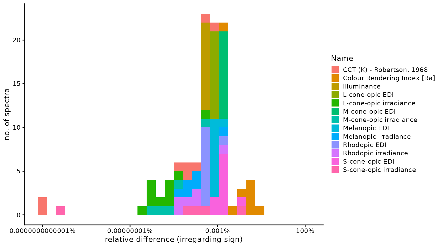
Base_Plot +
  scale_x_log10(breaks = breaks)+
  ylab("no. of spectra")+
  facet_wrap("Name")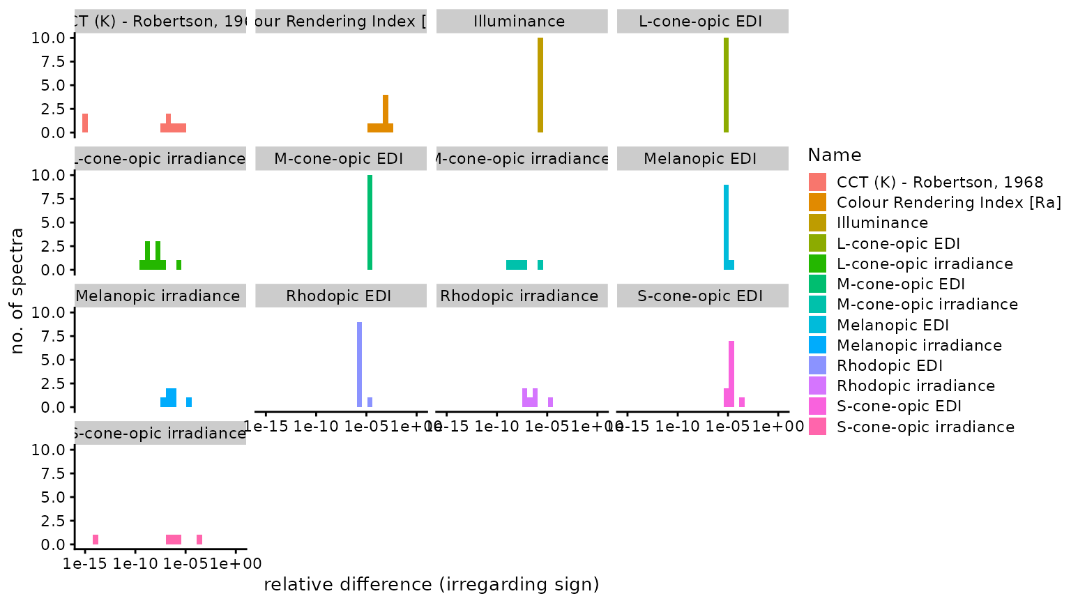
Base_Plot +
  scale_x_log10(breaks = breaks)+
  ylab("no. of variables")+
  facet_wrap("spectrum_name")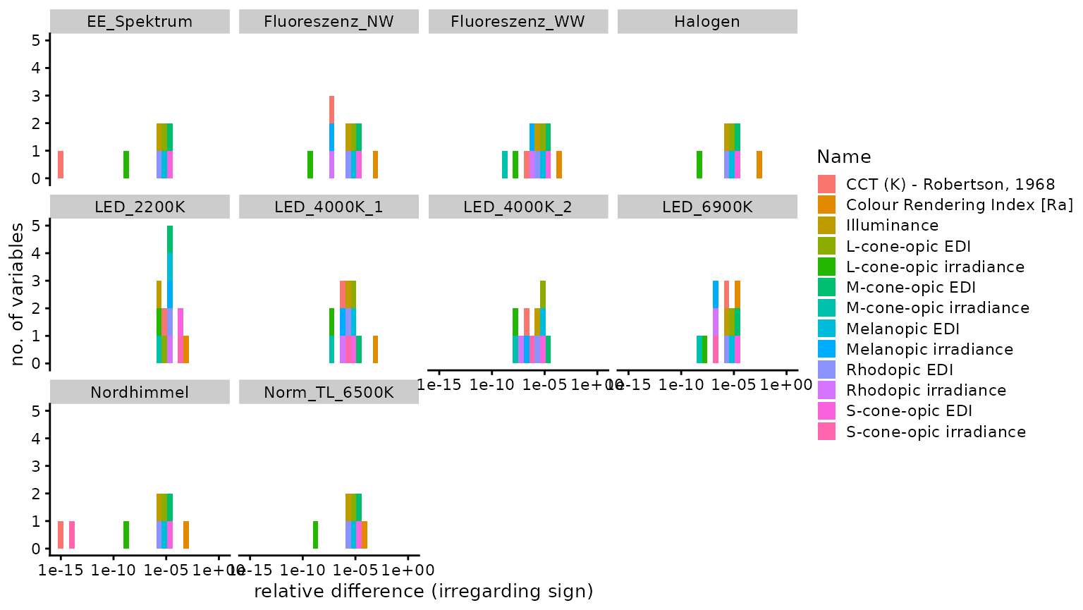
Pairwise comparison to the CIE Toolbox
CIE prep
#creating a subframe for the luox-data, filtered by removing all non-comparisons
Data <- Discussion %>% dplyr::filter(!is.na(Dev_toolbox))
#number of comparisons made
n <- Data %>% count() %>% pull(1)
#number of comparisons split by difference
n2 <- Data %>% group_by(Dev_toolbox == 0, Dev_toolbox > 0, Dev_toolbox < 0) %>%
  count() %>% pull(n)
n2[3] <- ifelse(is.na(n2[3]), "none",  n2[3])
#median difference when disregarding sign
n3 <- Data %>% filter(Dev_toolbox != 0) %>%
  dplyr::summarise(median = median(abs(Dev_toolbox))) %>% pull(1)
#maximum difference
n4 <- Data %>% pull(Dev_toolbox) %>% abs() %>% max()
#where did this difference occur
n4_2 <- Data$Name[abs(Data$Dev_toolbox) == n4]
Of 120 comparisons, none were identical, 25 were
smaller, and 95 were larger, using the
CIE Toolbox results as a basis. The median
relative difference was 1.13 × 10⁻⁶
(disregarding sign), i.e., 0.00011%. The highest relative
difference (again disregarding sign) was
1.81 × 10⁻⁵ or 0.0018%, which occured
for M-cone-opic EDI. The following figure provides a
histogram of all relative differences (excluding zero difference),
colored by variable.
Histogram
#make a histogram of the values and calculate relevant values

Base_Plot <-
  Data %>% filter(Dev_toolbox !=0) %>%
  ggplot(aes(x=abs(Dev_toolbox))) +
  geom_histogram(aes(fill = Name))+
  xlab("relative difference (irregarding sign)")+
  expand_limits(x= 1)
Base_Plot +
  scale_x_log10(breaks = breaks, labels = c(vec_fmt_number(breaks*100,
                                                           n_sigfig = 1,
                                                           pattern = "{x}%")))+
  ylab("no. of spectra")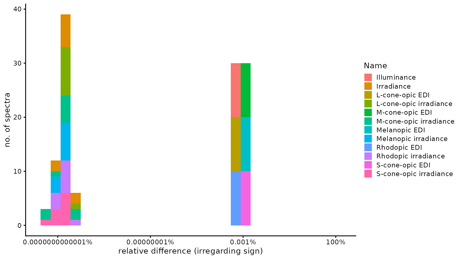
Base_Plot +
  scale_x_log10(breaks = breaks)+
  ylab("no. of spectra")+
    facet_wrap("Name")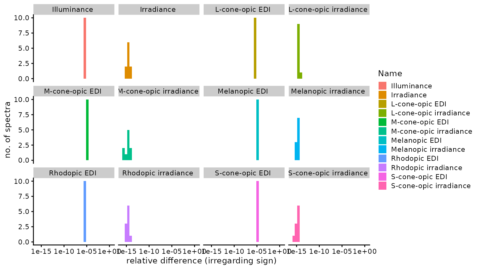
Base_Plot +
  scale_x_log10(breaks = breaks)+
  ylab("no. of variables")+
  facet_wrap("spectrum_name")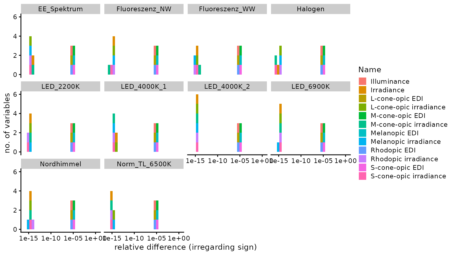
Conclusion
Overall, the agreement between the different sources is very high and
differences only occur several decimals back. For most if not all of
those cases, rounding errors seem a plausible explanation. In an older
version of the Shiny app, negative input values for
irradiance were taken at face value, i.e., they actually
reduced variable values that require summation. With that state, many
more comparisons showed a zero difference for the luox app,
which seems to indicate that the luox app also takes negative
values at face value. However, the median relative difference
in that older state was about double that compared to the current state
for both the luox app and the CIE Toolbox
sources. Since both the overall error is reduced by the current state of
the Shiny app and it is sensible to restrict input values
to zero or positive numbers, this method will be used in the public
release.
In summary, the Shiny app offers a sufficiently accurate
calculation of ⍺-opic values, especially given its focus on education.
It is of note, however, that the age corrected values could no be
validated against the other two sources, since they don´t provide
similar functionality.